How To Draw To Figure Different In Matlab

Plot Legends in MATLAB/Octave

Make your plots legendary

Plot legends are essential for properly annotating your figures. Luckily, MATLAB/Octave include the legend() function which provides some flexible and easy-to-employ options for generating legends. In this article, I embrace the basic apply of the legend() office, too as some special cases that I tend to use regularly.

The source code for the included examples can be found in the GitHub repository.

Basic Employ of Plot Legends

The fable() part in MATLAB/Octav e allows you to add together descriptive labels to your plots. The simplest mode to utilize the function is to pass in a character string for each line on the plot. The bones syntax is: fable( 'Clarification ane', 'Description ii', … ).

For the examples in this section, we will generate a sample figure using the following code.

          ten = 0 : 0.i : ( 2pi );            
plot( x, sin( x ), 'rx', 'linewidth', 2 );            
hold on;            
plot( ten, cos( x/3 ) - 0.25, 'bs', 'linewidth', 2 );            
plot( x, cos( 4x )/3, '^g', 'linewidth', 2 );
hold off;
xlim( [ 0, 2*pi ] );
filigree on;
championship( 'Sample Plot' );
prepare( gca, 'fontsize', 16 );

A legend can exist added with the following control.

          legend( 'Line 1', 'Line 2', 'Line three' );

In addition to specifying the labels as individual graphic symbol strings, it is oft convenient to collect the strings in a prison cell array. This is near useful when you are programmatically creating the fable string.

          legStr = { 'Line i', 'Line 2', 'Line three' };
legend( legStr );

For convenience, this method will be used for the balance of the examples. The resulting figure looks like this.

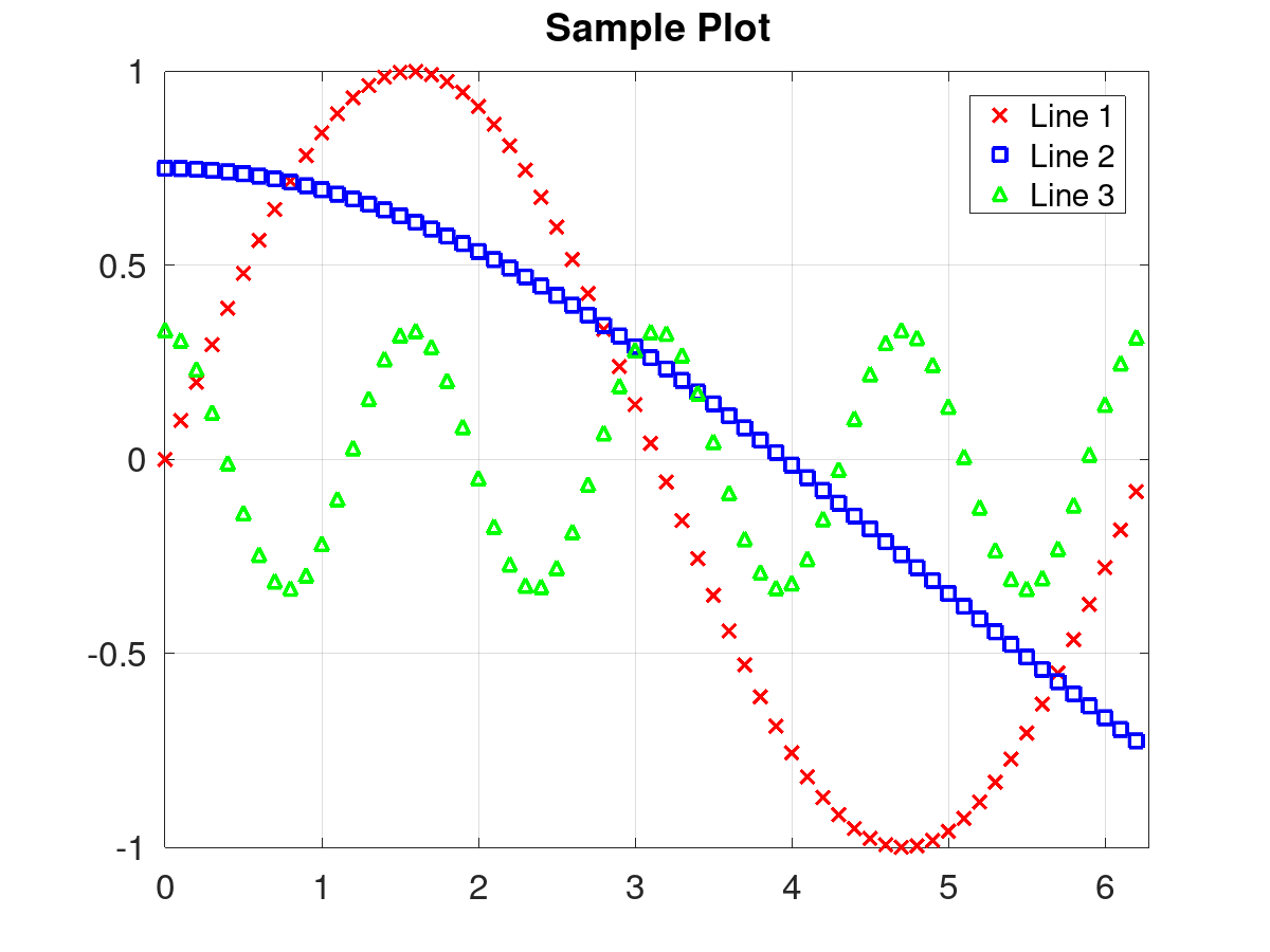
By default the legend has been placed in the upper, correct corner; however, the 'location' keyword tin be used to adjust where it is displayed. The location is selected using a convention based on the key directions. The post-obit keywords can be used: north, south, east, due west, northeast, northwest, southeast, southwest. The following code snippet would place the legend in the center tiptop of the plot.

          legend( legStr, 'location', 'northward' );

Similarly, all of the other keywords can be used to place the legend around the plot. The post-obit blitheness illustrates all of the different keywords.

The keyword 'outside' can besides be appended to all of the locations to identify the fable outside of the plot. The next image shows an example with the legend on the east exterior.

          legend( legStr, 'location', 'eastoutside' );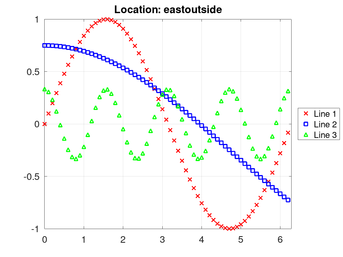

In addition to the setting the location, the legend() role also allows yous to gear up the orientation of the legend to either 'vertical' (default) or 'horizontal'. The following example volition position the legend at the bottom, outside of the plot, with a horizontal orientation.

          fable( legStr, 'orientation', 'horizontal', ...
            'location', 'southoutside' );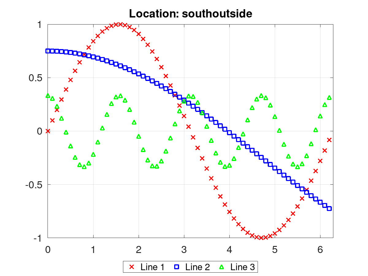

Using the "DisplayName" Property

Some other convenient way to add the legend labels is to set the "DisplayName belongings on the lines as they are plotted. This tin exist washed during the plot() telephone call or using set() on the handle. In both cases, afterwards yous have set the properties, you lot need to all legend() without any arguments to toggle the legend on.

The syntax for the plot() should wait like this.

          plot( x, sin( 10 ), 'rx', 'linewidth', ii, 'DisplayName', 'Line1' );
concord on;
plot( x, cos( x/iii ) - 0.25, 'bs', 'linewidth', 2, 'DisplayName', 'Line2' );
plot( x, cos( 4*x )/3, '^g', 'linewidth', ii, 'DisplayName',            
'Line3' );
hold off;

The syntax for the set up() should like this.

          % Plot the lines
h1 = plot( x, sin( x ), 'rx', 'linewidth', two, 'DisplayName', 'Line1' );
hold on;
h2 = plot( x, cos( x/3 ) - 0.25, 'bs', 'linewidth', ii, 'DisplayName', 'Line2' );
h3 = plot( x, cos( 4*ten )/3, '^grand', 'linewidth', 2, 'DisplayName', 'Line3' );
agree off;          % Update the brandish names
set( h1, 'DisplayName', 'Line1' );
set up( h2, 'DisplayName', 'Line2' );
set( h3, 'DisplayName', 'Line3' )

The legend would so be toggled on by calling legend() without any input arguments.

          legend();

The resulting plot would be the same as the get-go example shown earlier in the tutorial.

Using the Fable Handle

Similar to all of the other graphics objects, the fable properties can be adjusted using the fix() and get() functions. The post-obit lawmaking volition capture the legend handle and so set a few of the legend properties. In this particular example, the location is set to northeast, the orientation is set up to vertical, the font size is set to 16, and the box outline is removed.

          hl = fable( legStr );     % save the fable handle
set( hl, 'orientation', 'vertical' );     % set the orientation
gear up( hl, 'location', 'northeast' );     % gear up the location
set( hl, 'fontsize', xvi );     % set the font size
set up( hl, 'box', 'off' );    % plow off the box lines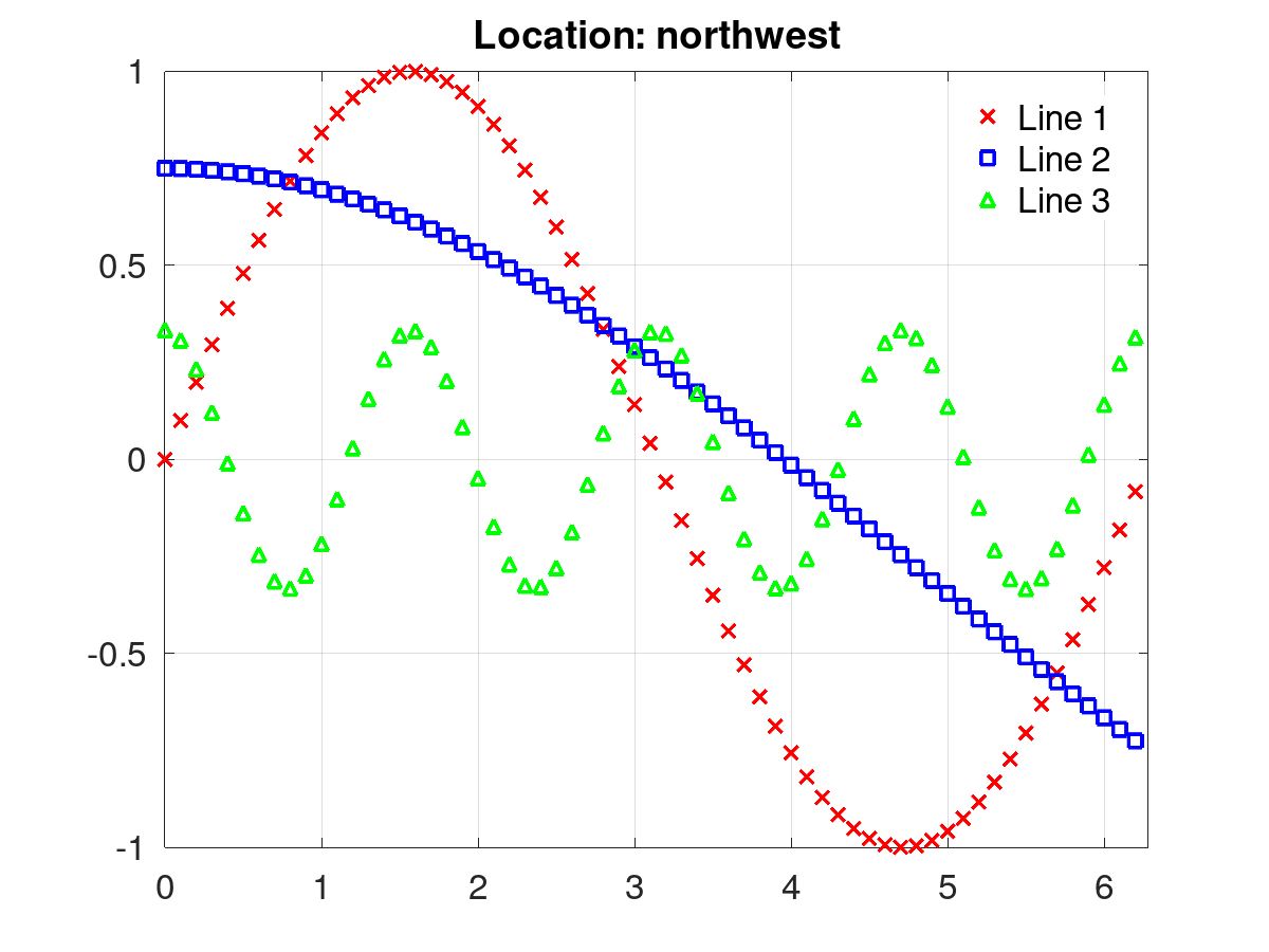

There are number of other backdrop that can be set on the legend object. Simply phone call get(hl) in the command window to display them all. One of the almost convenient of these properties is the 'position' belongings. The position property allows u.s. to gear up the exact position of the legend by specifying its horizontal origin (h0), vertical origin (v0), width (westward) and height (h). If you are not familiar with setting the position property on graphics object, you tin see a cursory description here.

Whenever you are working with subplots or GUIs, it is ofttimes necessary to specify an verbal location for the fable. This ensures that your fable does overlap with other elements or create weird spacing. Edifice on the previous example, we tin mock upward an instance GUI that includes our plot, a couple of buttons, and a legend that is manually placed on the figure.

          % Fix the subplot
set( f, 'units', 'normalized' );
a = subplot( 'position', [ 0.1, 0.ane, 0.five, 0.8 ] );          % Build our sample plot
x = 0 : 0.1 : ( two*pi );
plot( x, sin( x ), 'rx', 'linewidth', 2 );
hold on;
plot( x, cos( 10/iii ) - 0.25, 'bs', 'linewidth', 2 );
plot( x, cos( iv*ten )/three, '^g', 'linewidth', 2 );
agree off;
xlim( [ 0, 2*pi ] );
grid on;
championship( 'Sample Plot' );
gear up( a, 'fontsize', 16 );          % Add some buttons
a = uicontrol( f, 'units', 'normalized', 'position', [ 0.vii, 0.7, 0.ii, 0.1 ], ...
            'style', 'pushbutton', 'string', 'Printing Me' );
a = uicontrol( f, 'units', 'normalized', 'position', [ 0.7, 0.5, 0.2, 0.1 ], ...
            'fashion', 'pushbutton', 'string', 'Click Here' );          % Add together a legend manually
hl = legend( legStr );
set( hl, 'fontsize', sixteen );
prepare( hl, 'position', [ 0.74   0.25   0.12721   0.14310 ] );

Adding Specific Lines to the Fable

Rather than providing grapheme strings for all of the lines on the plot, information technology is possible to specify an assortment of specific line objects that should be included in the fable. I notice this especially useful for situations where you only need to draw attending to a few lines on the plot. I tend to apply this feature when I am plotting a large number of examples or realizations of some kind and want to overlay and highlight some statistics or metrics.

The post-obit case creates some random data and calculates some statistics from it. All of the realizations are plotted every bit thin gray lines and the statistics are overlaid as much thicker colored lines.

          % Generate some random data and calculate a few statistics
t = sqrt( 0.5 ) * randn( 100, 500 );
ts = sort( t, 2 );
t10 = ts( :, floor( 0.x * size( t, ii ) ) );
t90 = ts( :, floor( 0.ninety * size( t, 2 ) ) );          % Plot realizations as thin gray lines and statistics equally thicker, colored lines
plot( t, 'linewidth', 0.two, 'color', [0.5 0.five 0.5] );
concord on;
l1 = plot( mean( t, 2 ), 'linewidth', iv, 'colour', [0, 1, 0] );
l2 = plot( t10, 'linewidth', 4, 'color', [1, 0, 0] );
l3 = plot( t90, 'linewidth', 4, 'color', [0, 0, 1] );
hold off;
grid on;
ylim( [-3, iii] );
title( 'Statistics' );
set( gca, 'fontsize', 16 );          % Add a fable to just the statistics
hl = legend( [ l1, l2, l3 ], 'Mean', '10th Prct', '90th Prct', ...
            'orientation', 'horizontal', 'location', 'due north' );
ready( hl, 'fontsize', xvi );

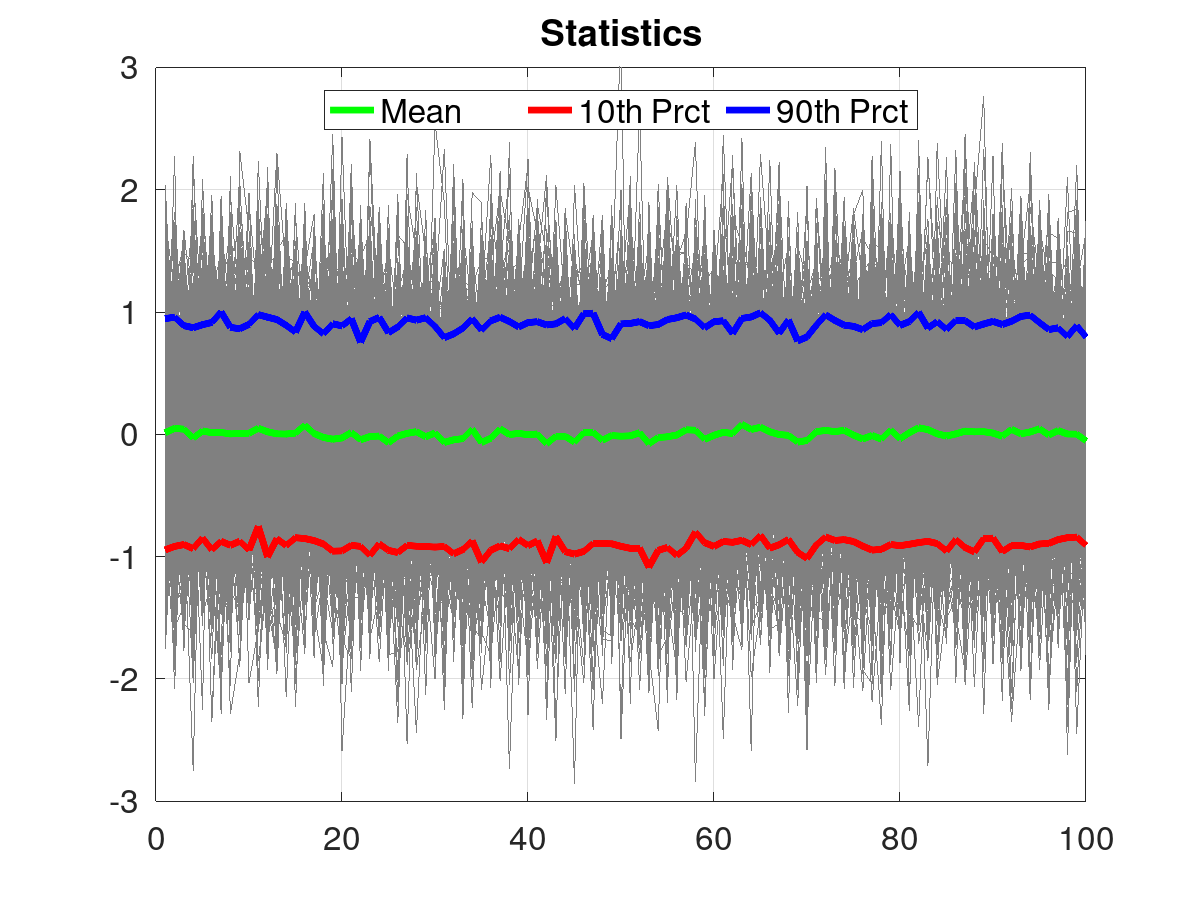
The consequence is a pretty nice plot (in my opinion). If we didn't pass in the line handles, so the fable() part would have tried to add a legend label to every unmarried realization. There are certainly other utilize cases; however, this is a type of plot that I tend to brand pretty frequently.

Summary

In this commodity, I covered several ways to use the legend() office in MATLAB/Octave. Here are a few key things to remember.

The legend labels tin be passed in as individual graphic symbol strings or as a cell array.
There a number of both position and orientation options that can be used to place the legend in certain parts of the figure.
The legend graphics handle can be used to directly ready any of the legend backdrop, including manually setting the position anywhere in the figure.
Line graphics handles tin can exist used to specify a subset of lines that volition be labeled in the legend.

Happy coding!